Implementing robust RAG pipelines: Integrating Google’s Gemma 2 (2B) open model, MongoDB, and LLM evaluation techniques

A step-by-step guide to implementing RAG for optimized query performance in MongoDB Atlas.

During the early days of the generative AI era, a period defined by the emergence of large language models (LLMs) capable of advanced response synthesis, reasoning, and planning capabilities, the observable trend was an increase in the number of parameters within newly released models. GPT-3 was released with 175 billion parameters in 2020, marking a significant leap from its predecessor, GPT-2, which had 1.5 billion parameters. This trend continued with even larger models like GPT-4, estimated to have over a trillion parameters, although OpenAI has yet to disclose the exact number publicly.

However, a counteracting effort was also taking place to reduce the sizes of these language models while maintaining the capabilities and qualities of similarly larger-sized LLMs. Google is a player on both sides of the language model sizing effort. Gemini is Google’s multimodal LLM, released in December 2023. Several versions were released after offering the emergent abilities of large language models that span billions of parameters and have extensive context window sizes for inputs to the LLM.

However, this tutorial’s key focus is Gemma 2, especially the variant with just two billion parameters.

As Google described, Gemma “is a family of lightweight, state-of-the-art open models” built with the same building blocks used to create the Gemini models. Small language and open models have their place in various use cases that call for efficiency, cost-effectiveness, privacy, and latency.

This tutorial covers building an asset management analyst assistant using Gemma 2. The assistant can analyze market reports stored in a MongoDB database based on user-provided queries, effectively augmenting some of an analyst’s responsibilities.

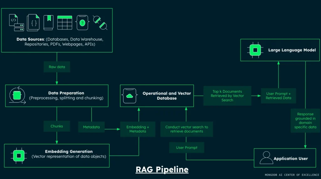
The tutorial also introduces the topic of LLM evaluation, specifically focusing on assessing key components in a typical retrieval-augmented generation (RAG) pipeline.

Read more: Getting started with Llamafile tutorial

What’s covered in this tutorial

• Building an asset management analyst assistant with Gemma 2
• Implementing a RAG pipeline with MongoDB
• Vector search and semantic retrieval techniques
• Generating responses using the Gemma 2 (2B) model
• LLM evaluation for RAG components

All code and implementation steps in this tutorial can be found on GitHub.

Step 1: Install libraries and set environment variables

The first step is to install all the libraries required to provide the functionalities to build the RAG pipeline components and conduct LLM evaluation for the retrieval and generation components of the RAG pipeline.

• PyMongo: Facilitates interaction with MongoDB databases
• Pandas: Provides powerful data manipulation and analysis capabilities
• Hugging Face (datasets): Offers access to a vast collection of pre-processed datasets
• Hugging Face (Sentence Transformers): Provides access to sentence, text, and image embeddings
• DeepEvals: Provides metrics for assessing LLM performance across various dimensions

Execute the following command to install and upgrade the required libraries:

!pip install --upgrade --quiet datasets pandas pymongo sentence_transformers deepevals

Setting up environment variables is crucial to ensuring secure access to external services. This practice enhances security by keeping sensitive information out of your codebase. Ensure you have a Hugging Face token(HF_TOKEN) in your development environment before running the code below.

import os
import getpass
# Make sure you have an Hugging Face token(HF_TOKEN) in your development environment before running the code below
# How to get a token: https://huggingface.co/docs/hub/en/security-tokens
os.environ["HF_TOKEN"] = getpass.getpass("Enter your Hugging Face token: ")
os.environ["OPENAI_API_KEY"] = getpass.getpass("Enter your OpenAI API key: ")  # Need this for the evaluation step

Step 2: Data loading and preparation

This step loads a financial dataset from Hugging Face into the current development environment. The data preparation process then creates a new attribute for each data point by combining several existing attributes. This combined attribute is prepared for the subsequent embedding generation step.

Data loading and preparation are processes in most data-related tasks and processing pipelines. Data loading refers to obtaining data from an external source and importing it into the current development environment for further downstream processing. Data preparation refers to organizing a dataset’s content in a format required for downstream processes. In this tutorial, data is loaded from the MongoDB Hugging Face organization.

The dataset is designed for financial analysis and market research in the tech sector. It provides a comprehensive view of each company, including news, financial metrics, and analyst reports. It could be used for tasks such as sentiment analysis, market trend analysis, or as part of a financial recommendation system.

import pandas as pd
from datasets import load_dataset

# Make sure you have an Hugging Face token(HF_TOKEN) in your development environment before running the code below
# How to get a token: https://huggingface.co/docs/hub/en/security-tokens
# https://huggingface.co/datasets/MongoDB/fake_tech_companies_market_reports
dataset = load_dataset("MongoDB/fake_tech_companies_market_reports", split="train", streaming=True)
dataset_df = dataset.take(100)

# Convert the dataset to a pandas dataframe
dataset_df = pd.DataFrame(dataset_df)
dataset_df.head(5)

Here are the steps taken in the code snippet above:

• The load_dataset function is used to fetch the "fake_tech_companies_market_reports" dataset from the MongoDB organization on Hugging Face.
• The "train" split is specified and is typically used for the main dataset in machine learning tasks.
• The streaming=True parameter is crucial here. It enables lazy dataset loading, allowing us to work with potentially very large datasets without loading everything into memory at once.
• dataset_df = dataset.take(100) uses the ‘take’ method to extract the first 100 samples from the dataset.
• After extracting a manageable subset of the data, we use Pandas to create a DataFrame object of the data for efficient data manipulation and visualization.
• We use Pandas’ "head" method to understand the dataset’s structure and content.

The operations above are steps taken to load data into the development environment and provide domain-specific data for the problem we are trying to solve. Specifically, we are creating a RAG-enabled chatbot that provides market information on tech-based companies for the asset management use case. The second half of this section focuses on data preparation.

A crucial part of the RAG pipeline process is data embedding, which creates a semantic representation of each data point that can be retrieved using information retrieval techniques such as vector search. Understanding which data attributes best capture the semantics, or in simpler terms, the meaning of a single data point, is crucial for building accurate and reliable RAG applications. Therefore, practitioners must carefully select and preprocess the most relevant features for embedding.

This involves:

• Conducting thorough exploratory data analysis to understand the dataset’s structure and content.
• Identifying key attributes that best represent the semantic essence of each data point.
• Considering domain-specific knowledge to guide feature selection and engineering.
• Evaluate and fine-tune the embedding process regularly to ensure it accurately captures the nuanced meanings and relationships within the data.

For our use case and this tutorial, the combination of the data attributes report, company, and sector suffices to capture the semantic detail of a data point. The code snippet below shows the operation of selecting the attributes and then defining the function combine_attributes to return the concatenated string of the selected attributes.

# Data Preparation
def combine_attributes(row):
 combined = f"{row['company']} {row['sector']} "

 # Add report information
 for report in row['reports']:
   combined += f"{report['year']} {report['title']} {report['author']} {report['content']} "

 # Add recent news information
 for news in row['recent_news']:
   combined += f"{news['headline']} {news['summary']} "

 return combined.strip()

The next process applies the combine_attributes to each datapoint in the dataset and stores the result of the operation in a new data point attribute: combined_attributes. This will be the attribute that is passed into the embedding model.

# Add the new column 'combined_attributes'
dataset_df['combined_attributes'] = dataset_df.apply(combine_attributes, axis=1)

Step 3: Embedding generation with GTE-Large

Be aware of the context window size of the embedding model you use. These models typically have a finite input capacity, often measured in tokens or characters. When input exceeds this threshold, the model may truncate the excess, potentially resulting in significant information loss. This truncation can severely impact the quality and relevance of the generated embeddings, compromising the overall performance of your RAG system.

If you have extensive data to embed, then it’s worth exploring varying chunking strategies. The standard advice for practitioners here is to implement chunking algorithms for longer documents that divide the text into semantically coherent segments, each fitting within the model’s context window and considering overlapping chunks to maintain contextual continuity.

For this use case and tutorial, the leveraged chunking strategy is to chunk any data that extends beyond the maximum input token length of the embedding model and attach the same metadata to the initial and secondary chunks.

The GTE (General Text Embeddings) model series, developed by the Institute for Intelligent Computing, Alibaba Group, provides state-of-the-art performance in text embedding technology. For this tutorial, we focus on using the GTE-Large English V1.5 model, which offers an optimal balance between performance and computational efficiency. This embedding model achieves a score of 65.39 on the Massive Text Embedding Benchmark (MTEB) for English, indicating overall embedding performance across a diverse set of NLP tasks and datasets. For the use case covered in this tutorial that involves information retrieval tasks, which means finding relevant documents for an input query, the GTE-Large English V1.5 model demonstrates a good performance with an average retrieval score of 57.91 based on an evaluation across 15 datasets.

from sentence_transformers import SentenceTransformer
from tqdm import tqdm
import numpy as np

# https://huggingface.co/thenlper/gte-large
# embedding_model = SentenceTransformer('thenlper/gte-large')
embedding_model = SentenceTransformer('Alibaba-NLP/gte-large-en-v1.5', trust_remote_code=True)

# Determine the maximum sequence length for the model
max_seq_length = embedding_model.max_seq_length

def chunk_text(text, tokenizer, max_length=8192, overlap=50):
  """
  Split the text into overlapping chunks based on token length.
  """
  tokens = tokenizer.tokenize(text)
  chunks = []
  for i in range(0, len(tokens), max_length - overlap):
      chunk_tokens = tokens[i:i + max_length]
      chunk = tokenizer.convert_tokens_to_string(chunk_tokens)
      chunks.append(chunk)
  return chunks

def get_embedding(text: str) -> list[float]:
  if not text.strip():
      print("Attempted to get embedding for empty text.")
      return []

  # Get the tokenizer from the model
  tokenizer = embedding_model.tokenizer

  # Split text into chunks if it's too long
  chunks = chunk_text(text, tokenizer, max_length=max_seq_length)
 
  if len(chunks) == 1:
      # If text fits in one chunk, embed as usual
      embedding = embedding_model.encode(text)
  else:
      # If text was split, embed each chunk and average the results
      chunk_embeddings = embedding_model.encode(chunks)
      embedding = np.mean(chunk_embeddings, axis=0)

  return embedding.tolist()

# Apply the embedding function with a progress bar
tqdm.pandas(desc="Generating embeddings")
dataset_df["embedding"] = dataset_df['combined_attributes'].progress_apply(get_embedding)

The code snippet above performs the following operations: Chunk the input data intended to be passed into the embedding model if it exceeds a particular length:

• Utilize the chunk_text function to tokenize and split long texts.
• Check the text split is within the model’s max_seq_length (8192 tokens for GTE-Large English V1.5).
• Implement an overlap of 50 tokens between chunks to maintain context continuity.

Pass the chunk(s) into the embedding model:

• For single chunks, directly encode using embedding_model.encode(text).
• For multiple chunks, encode each chunk separately.
• Handle potential empty inputs, returning an empty list if any empty inputs are present.

Store the embedding data as a new attribute embedding for each data point:

• Use tqdm to display a progress bar for all data points during the embedding process.
• Add the resulting embeddings as a new ’embedding’ column in the dataset_df DataFrame.
  

Read more: Harness the power of large language models part 1: Getting started with Ollama

Step 4: MongoDB vector database and connection setup

In this tutorial and many RAG applications, MongoDB acts as an operational and a vector database. MongoDB Atlas specifically provides a database solution that efficiently stores, queries, and retrieves vector embeddings.

Creating a database and collection within MongoDB is made simple with MongoDB Atlas.

1. First, register for a MongoDB Atlas account. Existing users can sign into MongoDB Atlas.
2. Follow the instructions. Select Atlas UI as the procedure to deploy your first cluster.
3. Create the database: asset_management_use_case.
4. Within the database asset_management_use_case, create the collection market_reports.
5. Create a vector search index named vector_index for the ‘listings_reviews’ collection. This index enables the RAG application to retrieve records as additional context to supplement user queries via vector search. Below is the JSON definition of the data collection vector search index.

Your vector search index created on MongoDB Atlas should look like the following:

{
 "fields": [
   {
     "numDimensions": 1024,
     "path": "embedding",
     "similarity": "cosine",
     "type": "vector"
   }
 ]
}

Follow MongoDB’s steps to get the connection string from the Atlas UI. After setting up the database and obtaining the Atlas cluster connection URI, securely store the URI within your development environment.

os.environ["MONGO_URI"] = getpass.getpass("Enter your MongoDB URI: ")

import pymongo

def get_mongo_client(mongo_uri):
"""Establish and validate connection to the MongoDB."""

client = pymongo.MongoClient(mongo_uri, appname="devrel.showcase.rag.cohere_mongodb.python")

# Validate the connection
ping_result = client.admin.command('ping')
if ping_result.get('ok') == 1.0:
  # Connection successful
  print("Connection to MongoDB successful")
  return client
else:
  print("Connection to MongoDB failed")
return None

MONGO_URI = os.environ["MONGO_URI"]

if not MONGO_URI:
print("MONGO_URI not set in environment variables")

mongo_client = get_mongo_client(MONGO_URI)

DB_NAME = "asset_management_use_case"
COLLECTION_NAME = "market_reports"

db = mongo_client.get_database(DB_NAME)
collection = db.get_collection(COLLECTION_NAME)

For this tutorial, to ensure we are working with a clean collection, you can run the code below to clear the collection of any existing data.

# Delete any existing records in the collection
collection.delete_many({})

Step 5: Data ingestion

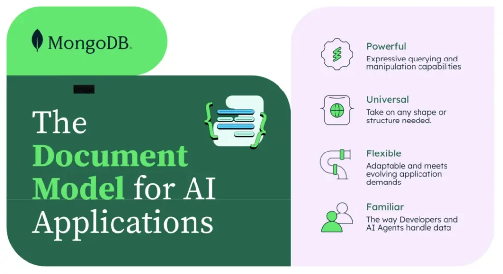
MongoDB’s document model and its compatibility with Python dictionaries offer several benefits for data ingestion. MongoDB’s document-oriented structure offers several advantages for data storage and manipulation in Python applications.The core of this structure is the use of BSON (Binary JSON) for data storage, which aligns naturally with Python’s dictionary data type. This alignment facilitates datarepresentation using key-value pairs, making it intuitive for Python developers to work with MongoDB.

One of MongoDB’s key features is its schema flexibility. Unlike traditional relational databases, MongoDB is schema-less, allowing each document in a collection to have a different structure. This flexibility is particularly advantageous in Python environments, as it complements Python’s dynamic nature. Developers can ingest varied data structures without predefined schemas, offering greater data handling and storage adaptability.

Another significant benefit of working with Python is MongoDB’s data ingestion efficiency. The close similarity between Python dictionaries and MongoDB documents enables direct data ingestion without complex transformations. This streamlined process results in faster data insertion and reduced processing overhead, making MongoDB an excellent choice for applications that require rapid data storage and retrieval in Python-based systems.

And that’s why the ingestion process within this tutorial is completed in one or two lines:

documents = dataset_df.to_dict('records')
collection.insert_many(documents)
print("Data ingestion into MongoDB completed")

Step 6: MongoDB query language and Vector Search

MongoDB’s query language is designed to work well with document structures, making it easy to query and manipulate ingested data using familiar Python-like syntax. The query language is executed using MongoDB’s aggregation pipeline, a powerful feature that allows for complex data processing and analysis within the database.

An aggregation pipeline can be thought of similarly to pipelines in data engineering or machine learning, where processes operate sequentially. Each stage takes an input, performs operations, and provides an output for the next stage.

Stages are the building blocks of an aggregation pipeline. Each stage represents a specific data transformation or analysis operation. Common stages include:

• $match: Filters documents (similar to WHERE in SQL)
• $group: Groups documents by specified fields
• $sort: Sorts the documents
• $project: Reshapes documents (select, rename, compute fields)
• $limit: Limits the number of documents
• $unwind: Deconstructs array fields
• $lookup: Performs left outer joins with other collections

The code snippet below defines a vector search function demonstrating semantic search implementation using MongoDB’s vector search capabilities. At its core, the function leverages dense vector embeddings to find documents semantically similar to a user’s query. It begins by converting the input query into a vector embedding, then utilizes MongoDB’s $vectorSearch operator to search through a pre-indexed collection of document embeddings efficiently.

def vector_search(user_query, collection):
"""
Perform a vector search in the MongoDB collection based on the user query.

Args:
user_query (str): The user's query string.
collection (MongoCollection): The MongoDB collection to search.

Returns:
list: A list of matching documents.
"""

# Generate embedding for the user query
query_embedding = get_embedding(user_query)

if query_embedding is None:
  return "Invalid query or embedding generation failed."

# Define the vector search pipeline
vector_search_stage = {
  "$vectorSearch": {
    "index": "vector_index",
    "queryVector": query_embedding,
    "path": "embedding",
    "numCandidates": 150,  # Number of candidate matches to consider
    "limit": 2  # Return top 4 matches
  }
}

unset_stage = {
  "$unset": "embedding"  # Exclude the 'embedding' field from the results
}

project_stage = {
  "$project": {
    "_id": 0,  # Exclude the _id field
    "company": 1,  # Include the plot field
    "reports": 1,  # Include the title field
    "combined_attributes": 1, # Include the genres field
    "score": {
      "$meta": "vectorSearchScore"  # Include the search score
    }
  }
}

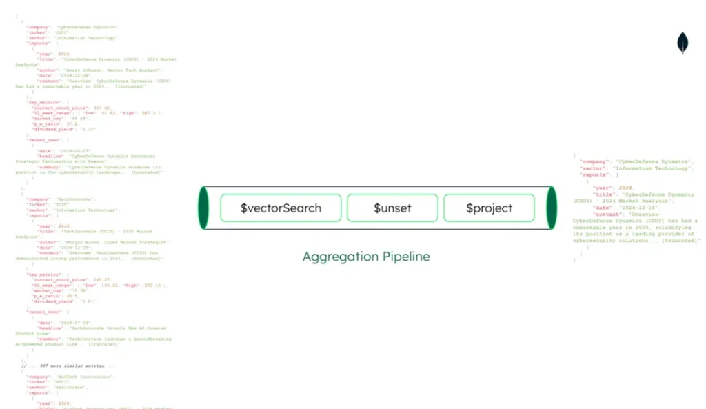
pipeline = [vector_search_stage, unset_stage, project_stage]

# Execute the search
results = collection.aggregate(pipeline)
return list(results)

The code snippet above does the following operations:

• Converts the user’s text query into vector embedding using the get_embedding function, which leverages the earlier embedding operations defined earlier
• Utilizes MongoDB’s $vectorSearch operator to find semantically similar documents
• Searches the vector_index using the query embedding; ensures that the vector search index has been created on MongoDB atlas and is referenced in the query using the name specified at creation
• Sets numCandidates to 150 for broad initial matching
• Limits the final results to the top two matches
• Uses an $unset stage to remove the “embedding” field from results, reducing data transfer
• Uses a $project stage to selectively include relevant fields: “company”, “reports”, and “combined_attributes”
• Adds a similarity score using $meta: "vectorSearchScore"
• Combines the stages into a single aggregation pipeline
• Executes the search using collection.aggregate()
• Returns the results as a list of documents

Step 7: Handling user queries

The next step after creating the information retrieval component aspect of the RAG pipeline is to handle the result, which means essentially formatting the retrieved documents in a manner that is consumable by the LLM in the generation step of the RAG pipeline.

In the code snippet below, the get_search_result function serves as a wrapper for the vector search operation, transforming raw search results into a more user-friendly format. The function returns a formatted string containing summarized information from the top search results.

def get_search_result(query, collection):

get_knowledge = vector_search(query, collection)

search_result = ''
for result in get_knowledge:
    search_result += f"Company: {result.get('company', 'N/A')}, Combined Attributes: {result.get('combined_attributes', 'N/A')}\n"

return search_result

The next step is to actually define an input query for the RAG pipeline. This input query is similar to what is expected for chatbot interfaces that expect prompts or inputs from users and provide a response. For the use case in this tutorial, the code snippet below demonstrates the practical application of the semantic search functionality in a question-answering context.

# Conduct query with the retrieval of sources
query = "What companies have negative market reports or negative sentiment that might deter from investment in the long term"
source_information = get_search_result(query, collection)
combined_information = f"Query: {query}\nContinue to answer the query by using the Search Results:\n{source_information}."

print(combined_information)

Step 8: Load Gemma 2 (2B)

This section of the tutorial demonstrates the initialization of Gemma 2.0 (2B), a two billion-parameter open language model and its associated tokenizer. This particular variant of the model is instruction-tuned, which means it has been specifically fine-tuned on a dataset of instructions and responses, enhancing its ability to understand and follow user prompts accurately.

The code snippet below uses the Hugging Face transformers library to load the tokenizers and model for the Gemma-2.0-2b, using the AutoTokenizer and AutoModelForCausalLM modules of the library. The tokenizer converts text into tokens that can be passed as inputs to be processed by the model.

import torch
from transformers import AutoTokenizer, AutoModelForCausalLM

tokenizer = AutoTokenizer.from_pretrained("google/gemma-2-2b-it")
model = AutoModelForCausalLM.from_pretrained("google/gemma-2-2b-it", torch_dtype=torch.bfloat16)

The code snippet below extracts the response from the Gemma 2 (2B) model.

def extract_model_response(response):
# Split the response at the start of the model's turn
parts = response.split("<start_of_turn>model")
 # If there's a model response, it will be in the last part
if len(parts) > 1:
  model_response = parts[-1].strip()
 
  # Remove any potential end-of-turn markers
  model_response = model_response.split("<end_of_turn>")[0].strip()
 
  return model_response
else:
  return "No model response found."

After initializing the Gemma 2.0 (2B) model and its associated tokenizer, the next step is to generate a response using a chat-style input format. This tutorial leverages the model’s chat template functionality to create a more conversational experience. The Gemma model tokenizer’s apply_chat_template method is utilized to properly format the input for the instruction-tuned model.

chat = [
  { "role": "user", "content": combined_information },
]
prompt = tokenizer.apply_chat_template(chat, tokenize=False, add_generation_prompt=True)

inputs = tokenizer.encode(prompt, add_special_tokens=False, return_tensors="pt")
outputs = model.generate(input_ids=inputs.to(model.device), max_new_tokens=150, do_sample=True, temperature=0.7)

response = tokenizer.decode(outputs[0])

The code snippet above performs the following operations:

1. Creation of chat-style input: A single user message containing the combined_information is formatted as a chat-style input.
2. Application of chat template: The tokenizer’s apply_chat_template method formats this input according to Gemma’s specific chat template. This process includes adding a generation prompt to guide the model’s response.
3. Tokenization and encoding: The formatted prompt is tokenized and encoded, preparing it for input into the model.
4. Response generation: The model generates a response using specified parameters, such as maximum_new_tokens and temperature. These parameters control the length and randomness of the output.
5. Decoding and extraction: Finally, the generated output is decoded and processed to extract the model’s response, making it ready for response extraction and other downstream processes.

model_output = extract_model_response(response)
print(model_output)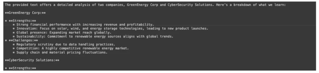

Step 9: LLM evaluation

LLM evaluation, also referred to as LLM evals, is the systematic process of formulating a profile of foundation models or their derived fine-tuned variants to understand and capture their performance on certain specialized or general-purpose tasks, reliability in certain conditions, effectiveness in particular use cases, and many other evaluative measurement criteria that help in gaining an overview of a model’s overall ability.

The particular category of LLM evaluation performed in this tutorial is LLM system evaluation, defined as the end-to-end performance overview of a system or infrastructure that incorporates an LLM; examples of such systems are RAG pipelines and agentic systems.

Although the RAG pipeline has multiple components, this tutorial will only evaluate the generation component. The generation component involves using the retrieved relevant information from the database to produce a coherent and accurate response to the user’s query. Specifically, it includes:

1. Integrating the retrieved context(source_information) with the original query (query).
2. Prompting the language model with this combined information (combined_information).
3. Generating a response(model_output) that addresses the user’s question or request.
4. Ensuring the generated content is relevant, coherent, and faithful to the retrieved information. This is what we are doing in this section.

This component is crucial as it determines the final output quality of the RAG system, directly impacting user experience and the system’s overall effectiveness. The evaluation metrics and factors for the generation component of a RAG pipeline are relevancy, faithfulness, coherence, and accuracy.

The LLM evaluation framework leveraged in this tutorial is DeepEval. DeepEval provides the evaluation metrics: answer relevance, faithfulness, hallucination, and others, as well as the ability to define custom metrics. This tutorial will utilize just two metrics: answer relevance and faithfulness.

Faithfulness: Faithfulness quantifies the extent to which the factual information in the generated text aligns with the retrieved documents or provided context. Faithfulness is measured in the DeepEval library by using an LLM to extract claims that are made in the model’s response to a user query and provided context and then using the same LLM to determine if the claims extracted from the model’s response are observed in the retrieved context. Therefore, the faithfulness score is determined by the number of “backed” claims in the model’s response divided by the total number of claims in the model’s response.

faithfulness = (Number of truthful claims) / (Total number of claims in response)

To begin the evaluation step, ensure that the DeepEval Python library is installed within your development environment. Next, import the LLMTestCase and FaithfulnessMetric modules from the DeepEval library.

• LLMTestCase
• FaithfulnessMetric

from deepeval.test_case import LLMTestCase
from deepeval.metrics import FaithfulnessMetric

from deepeval.metrics import FaithfulnessMetric

actual_output = model_output

retrieval_context = [source_information]

metric = FaithfulnessMetric(
  threshold=0.7,
  model="gpt-4",
  include_reason=True
)
test_case = LLMTestCase(
  input=query,
  actual_output=actual_output,
  retrieval_context=retrieval_context
)

metric.measure(test_case)
print(metric.score)
print(metric.reason)

The code snippet above sets up variables actual_output and retrieval_context to store the model’s output and the source information for context. A FaithfulnessMetric object is instantiated with a threshold of 0.7, corresponding to the faithfulness boundary, resulting in a flagging in the evaluation output for claims that fall below the threshold.

The evaluation procedure uses “GPT-4” as the evaluation model and is configured to include a reason for its assessment, using the LLM as a judge approach for evaluation. An LLMTestCase is constructed, encompassing the input query, the model’s actual output, and the retrieval context. The code snippet shows the invocation of the metric’s measure method, passing the test case as an argument. Finally, the code snippet outputs the calculated faithfulness score and the accompanying explanation for the evaluation.

Below is an example of the output of the faithfulness evaluation process.

Event loop is already running. Applying nest_asyncio patch to allow async execution...
0.9333333333333333
The score is 0.93 because there is a minor discrepancy with the year of CDDY's strategic acquisitions. The actual output mistakenly indicates they occurred in 2023, while the context clearly states they happened in 2024.

The faithfulness score is 0.93, which can be interpreted as Gemma 2B’s response being 93% faithful to the provided context. The accompanying explanation also provides a reason for the provided score, a response generated by the LLM used for evaluation to provide a textual explanation of its result. This component of the DeepEval library introduces a human-readable explanation feature, which enhances the interpretability of the evaluation results. It provides a clear rationale for the faithfulness score, highlighting discrepancies or alignments between the model’s output and the source context.

Answer relevance: This quantifies how well the generated response aligns with the initial input query. Answer relevance assesses the association between the response and the query without evaluating factual accuracy.

from deepeval.metrics import AnswerRelevancyMetric

actual_output = model_output

metric = AnswerRelevancyMetric(
  threshold=0.7,
  model="gpt-4",
  include_reason=True
)

test_case = LLMTestCase(
  input=query,
  actual_output=actual_output
)

metric.measure(test_case)
print(metric.score)
print(metric.reason)

The result of the answer relevance evaluative process is as follows:

Event loop is already running. Applying nest_asyncio patch to allow async execution...
1.0
The score is 1.00 because the response accurately selected a company from the provided information and justified why it's a safe long-term investment, addressing all aspects of the input.

In this section, you were introduced to LLM evaluation, specifically focusing on LLM system evaluation within the context of a RAG pipeline. You implemented two key evaluative methods for the generation component of a RAG pipeline: answer relevance and faithfulness, utilizing the powerful deepevals library.

By leveraging the DeepEval library, you could quantify these aspects of the model’s performance and gain valuable insights into its strengths and areas for improvement. The library’s ability to provide numerical scores and human-readable explanations enhances the interpretability of your evaluation results.

Moving forward, you can explore the other evaluative metrics the DeepEval library offers.

Conclusion

In this tutorial, you explored building an asset management analyst assistant using Google’s Gemma 2 (2B) open model, a RAG pipeline with MongoDB, and LLM evaluation techniques. This showcase demonstrates the potential of open models in creating efficient, cost-effective AI solutions for specific use cases.

The implementation of Gemma 2 (2B), a lightweight two billion-parameter model, highlights the growing capabilities of open-source models in real-world applications and environments with limited compute availability. This allows developers to create AI-driven solutions that balance performance with resource efficiency.

MongoDB’s operational and vector database role underscores its flexibility and scalability in modern AI applications and infrastructure. Its vector search capabilities and Python integration make it well-suited for RAG systems, enabling efficient information retrieval.

The focus on LLM evaluation using the DeepEval library emphasizes the importance of assessing AI system performance. By implementing metrics like faithfulness and answer relevance, you gained insights into the model’s strengths and areas for improvement.

Moving forward, you can explore more evaluation approaches or chunking strategies to optimize the performance and accuracy of RAG pipelines.

Get the full code for this tutorial.

FAQs

1. What is Gemma 2, and how does it differ from other language models?

Gemma 2 is a family of lightweight, state-of-the-art open models developed by Google. It’s built using the same building blocks as the larger Gemini models but is designed to be more efficient and suitable for use cases that require lower computational resources. The Gemma 2 (2B) variant has two billion parameters and is particularly useful for applications that need efficiency, cost-effectiveness, privacy, and low latency.

2. How does MongoDB contribute to the RAG pipeline?

MongoDB serves as both an operational and vector database in this RAG application. It efficiently stores, queries, and retrieves vector embeddings. The tutorial demonstrates how to set up a MongoDB Atlas cluster, create a vector search index, and use MongoDB’s aggregation pipeline for semantic search capabilities, which are crucial for the retrieval component of the RAG system.

3. What is LLM evaluation, and which metrics are used in this tutorial?

LLM evaluation, or LLM evals, is the systematic process of assessing language models’ performance on various tasks and use cases. In this tutorial, the focus is on LLM system evaluation, specifically for a RAG pipeline. Two key metrics are used: faithfulness and answer relevance. Faithfulness measures how well the generated response aligns with the provided context, while answer relevance assesses how well the response addresses the initial query.

4. What is the purpose of the DeepEval library in this tutorial?

The DeepEval library is used to conduct LLM evaluations. It provides metrics such as FaithfulnessMetric and AnswerRelevancyMetric to assess the quality of the generated responses. The library allows for setting evaluation thresholds and using models like GPT-4. It includes features for providing human-readable explanations of the evaluation results, enhancing the interpretability of the assessment process.

More from We Love Open Source

• Building a RAG system with Google’s Gemma, Hugging Face, and MongoDB
• Harness the power of large language models part 1: Getting started with Ollama
• Harness the power of large language models part 2: Working with Ollama
• How Netflix uses an innovative approach to technical debt
• How to get involved with We Love Open Source

This article is adapted from “Implementing Robust RAG Pipelines: Integrating Google’s Gemma 2 (2B) Open Model, MongoDB, and LLM Evaluation Techniques” by Richmond Alake, and is republished with permission from the author.